Why your Excel formula is not working, and how to fix it
An Excel formula usually fails in one of two ways. Either Excel refuses it and shows an error such as #NAME? or #REF!, or it calculates without complaint and gives the wrong answer. The second kind is the dangerous one, because nothing tells you it is wrong. This guide covers the causes we see most often on our practice site, what each error code means, and how to fix the formula.
Absolute and relative references: when to use the $ sign
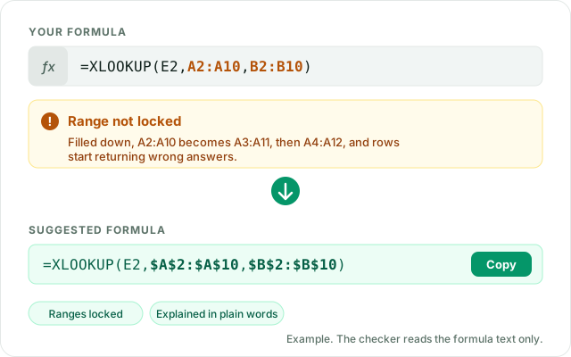
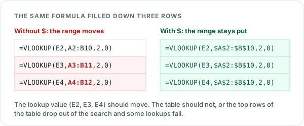
When you copy or fill a formula, Excel moves every cell reference by the same amount. That is right for the value you are looking up, but wrong for a lookup table, which should stay in place. A $ fixes part of a reference: $A$2 never moves, A$2 keeps the row, and $A2 keeps the column. While editing a reference, press F4 to cycle through the four options. The checker flags lookup and condition ranges in functions such as XLOOKUP, VLOOKUP, MATCH, INDEX, SUMIFS and COUNTIFS that have no $ at all.
Why VLOOKUP returns the wrong value
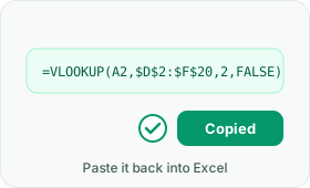
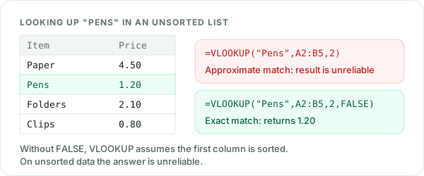
VLOOKUP and HLOOKUP have a fourth argument that is easy to leave out. Without it, they use approximate match, which assumes the first column is sorted and returns the closest value below the one you asked for. On unsorted data, such as product codes or names, the answer is unreliable. Add FALSE (or 0) as the fourth argument for an exact match. MATCH has the same trap: its third argument defaults to approximate, so use 0. XLOOKUP and XMATCH use exact match by default.
How to fix the #NAME? error
#NAME? means Excel does not recognise something in the formula. Check for a misspelt function (VLOKUP), text without quotation marks, a named range that does not exist, or curly quotes (“ ”) copied from a web page or a document, which Excel does not accept. A function that your version of Excel does not have, such as XLOOKUP in Excel 2016, also shows #NAME?. The checker straightens curly quotes and corrects one-letter slips in function names.
Why a lookup returns #N/A when the value is there
#N/A means the lookup value was not found. When you can see the value in the list, the two are usually not exactly equal: one has a trailing or non-breaking space, or one is a number and the other is a number stored as text. A lookup range that moved because it was not locked has the same effect for rows near the top. Clean the data first (the Data Cleaner trims spaces and converts text to numbers), lock the range, and use IFNA or IFERROR only once you know why values are missing.
How to fix the #REF! error
#REF! means a reference points to a cell that does not exist. Two common causes: a VLOOKUP column number larger than the number of columns in the table (asking for column 4 of D2:F20), and a formula whose source cells, rows or sheet were deleted. The checker catches the first. For the second, undo the deletion or rewrite the reference.
How to fix the #VALUE! error
#VALUE! appears when a function gets the wrong type of value or ranges that do not line up. In SUMIFS, COUNTIFS and similar functions every range must be the same size, and in XLOOKUP the lookup and return ranges must have the same number of rows (or columns). Arithmetic on text, such as adding a cell that contains a space, also gives #VALUE!.
How to fix the #DIV/0! error
#DIV/0! means the formula divided by zero or by an empty cell. If an empty divisor is expected, wrap the formula: =IFERROR(A2/B2,0), or test first with =IF(B2=0,"",A2/B2). Do not hide the error if the divisor should never be zero; find out why it is.
Missing brackets and commas versus semicolons
Every opening bracket needs a closing one, and Excel will not accept the formula until they match. The checker counts them and adds missing closing brackets at the end, but check that is where they belong in a nested formula. In many European regional settings Excel separates arguments with semicolons (=IF(A1>0;1;2)) instead of commas. A formula copied between the two settings will not work; the checker suggests commas, which is right for English (US or UK) settings.
How to check a formula inside Excel
Excel has its own tools on the Formulas tab, in the Formula Auditing group. Error Checking walks through cells that show errors. Evaluate Formula calculates a formula one step at a time so you can see where it goes wrong. Trace Precedents draws arrows to the cells a formula uses, and Show Formulas (Ctrl+`) displays formulas instead of results. In the formula bar, select part of a formula and press F9 to see its value, then press Esc so the formula is not changed.
Excel error codes at a glance
| Error | What it means | Usual fix |
|---|---|---|
#NAME? | Excel does not recognise a name | Check spelling, quotes and your Excel version |
#N/A | The lookup value was not found | Clean spaces and types, lock the range |
#REF! | A reference points nowhere | Check column numbers and deleted cells |
#VALUE! | Wrong type of value or mismatched ranges | Make ranges the same size, remove text from maths |
#DIV/0! | Division by zero or an empty cell | Use IF or IFERROR, or fix the divisor |
| Wrong answer, no error | Approximate match or a moved range | Add FALSE or 0, add $ signs |
To practise these functions on exercises that tell you why an answer is wrong, try Excel Practice Sheets. For date formulas, see the Date Helper.
Questions about Excel formula errors
How do I check an Excel formula for errors?
Paste the formula into the checker above to see likely mistakes with a fixed version. Inside Excel, use the Formulas tab: Error Checking lists cells with errors, Evaluate Formula steps through a calculation, and Trace Precedents shows which cells feed the formula.
Why does my formula show #NAME?
Excel does not recognise something in the formula. The usual causes are a misspelt function name, text without quotation marks, curly quotes copied from a web page, or a function that your version of Excel does not have.
Why does VLOOKUP return the wrong value?
Most often the last argument is missing, so VLOOKUP uses approximate match and expects the first column to be sorted. Add FALSE as the fourth argument for an exact match. Also check that the table range is locked with $ signs if the formula is filled down.
What does the $ sign mean in an Excel formula?
A $ fixes the column or row of a reference so it does not change when the formula is copied. $A$2 always points to A2, A$2 keeps the row fixed, and $A2 keeps the column fixed. Press F4 while editing a reference to cycle through these.
Why does my lookup return #N/A when the value is there?
The two values are not exactly equal. Common reasons are extra or non-breaking spaces, a number stored as text in one place and as a number in the other, or a lookup range that has moved because it was not locked.
Are my formulas uploaded?
No. The checker runs in your browser. Nothing you paste is sent to a server or stored.
Is the Formula Checker always right?
No. It reads only the formula text, not your workbook, so it points out likely mistakes rather than proving a formula is correct. Some findings are questions about what you meant, and those are never changed automatically.